The XLOOKUP Function in Excel
The XLOOKUP function in Excel is newly introduced in the latest version of Excel, which is a powerful replacement for older lookup functions like VLOO...
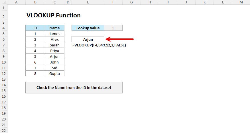
The VLOOKUP function in Excel looks for a value in the first column of a table and gives you back information from another column in the same row.
=VLOOKUP(lookup_value, table_array, col_index_num, [range_lookup])When VLOOKUP finds what you're looking for, it gives you back the information from the column you asked for. If it can't find anything and you used FALSE, you'll get an error message.
VLOOKUP helps you find information quickly from big lists of data. Think of it like asking someone to look up a phone number for you - you give them a name, and they find the number. You can use it for employee information, product prices, customer details, or any time you need to match one piece of information with another.
You have a list of employees and want to find someone's department by typing their employee ID.
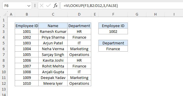
=VLOOKUP(F3,B2:D12,3,FALSE)When you type an employee ID in cell F3, this formula looks for that ID in column B and gives you back the department from column 3. We are using FALSE here because we want an exact match to be returned.
You're making an invoice and need to find product prices automatically when you enter product codes.
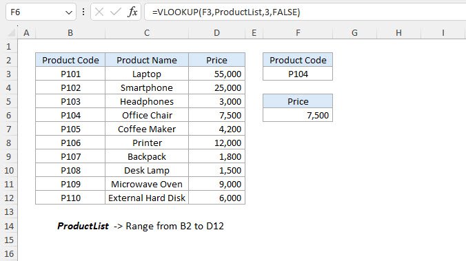
=VLOOKUP(F3,ProductList,3,FALSE)Type a product code in F3, and this formula finds that code in your product list and shows you the price from column 3. This saves time and prevents mistakes.
A teacher wants to turn number scores into letter grades using a grade scale.
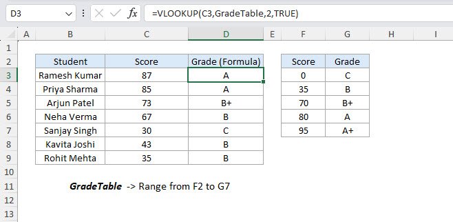
=VLOOKUP(C3,GradeTable,2,TRUE)This formula looks at a student's score and finds the right grade level. We use TRUE because we want the closest match - if someone gets 87, it should find the A grade range.
A sales team gets different commission rates based on how much they sell.
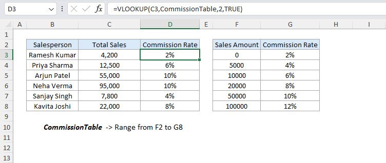
=VLOOKUP(C3,CommissionTable,2,TRUE)This looks at how much someone sold and finds their commission rate. Using TRUE helps it find the right rate level even if the exact sales amount isn't in the table.
If you want to learn how to create named ranges in Excel, read this blog.
You want to show "Not Found" instead of error messages when someone types a wrong employee ID.
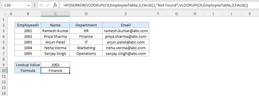
=IF(ISERROR(VLOOKUP(C9,EmployeeTable,3,FALSE)),"Not Found",VLOOKUP(C9,EmployeeTable,3,FALSE))The IF function checks if VLOOKUP finds an error. If there's an error, it shows "Not Found". If everything works fine, it shows the employee information.
You want to make your spreadsheet look professional by hiding error messages.
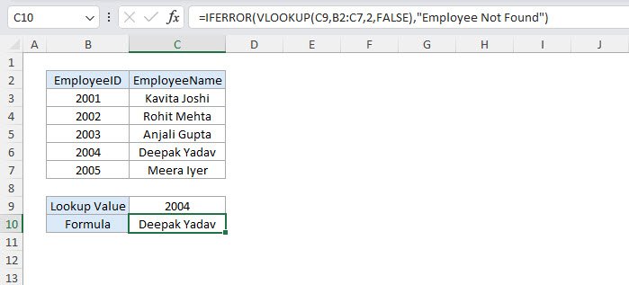
=IFERROR(VLOOKUP(C9,B2:C7,2,FALSE),"Employee Not Found")IFERROR is easier to use than IF. It catches any problems with VLOOKUP and shows your own message instead of confusing error codes.
You need to search for employees using their full name, but your data has first and last names in separate columns.
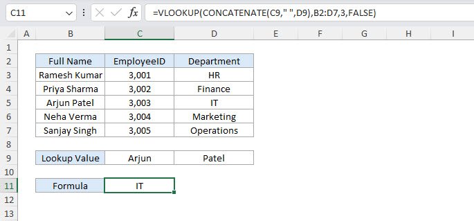
=VLOOKUP(CONCATENATE(C9," ",D9),B2:D7,3,FALSE)CONCATENATE puts the first name and last name together with a space, then VLOOKUP uses that combined name to find the employee information.
VLOOKUP makes it easy to find and show data from big tables. It helps you find information quickly from large amounts of data, whether you're working with employee records, product catalogues, or customer information. Remember to use FALSE for exact matches most of the time, and add error handling to make your spreadsheets look more professional.
No comments yet. Be the first to comment!
Free offline Android app to learn Excel formulas, functions & shortcuts anytime, anywhere!
Download Free AppPress Ctrl+1 to open Format Cells dialog for any selected range.