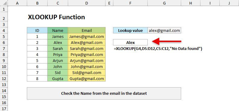
The XLOOKUP Function in Excel
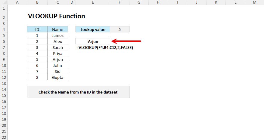
The XLOOKUP function in Excel is newly introduced in the latest version of Excel, which is a powerful replacement for older lookup functions like VLOO...
Sep 08, 2025
Read More