The XLOOKUP Function in Excel
The XLOOKUP function in Excel is newly introduced in the latest version of Excel, which is a powerful replacement for older lookup functions like VLOO...
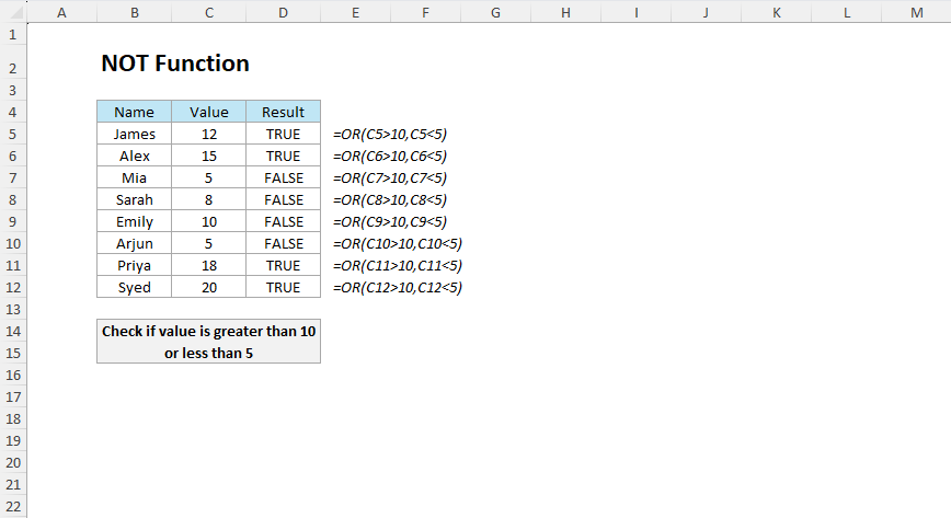
The NOT function in Excel is a useful function when you want to reverse a logical value by returning TRUE if the condition is FALSE and FALSE if the condition is TRUE.
=NOT(logical)The NOT function reverses the logical value: if the logical test returns TRUE, NOT will return as FALSE or vice versa by reversing the output.
The NOT function is majorly used when you want to exclude specific conditions or to reverse the logic in decision-making, data validation, and conditional formatting. It easily pairs with other functions like IF, AND, and OR to create complex logical tests.
A teacher wants to identify students who have not submitted their assignments.
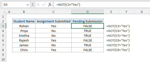
=NOT(C3="Yes")The formula checks if the Assignment Submitted column does not contain Yes. For Priya, the result is TRUE because the assignment was not submitted by her.
A logistics manager tracks deliveries and wants to flag items not delivered on time.
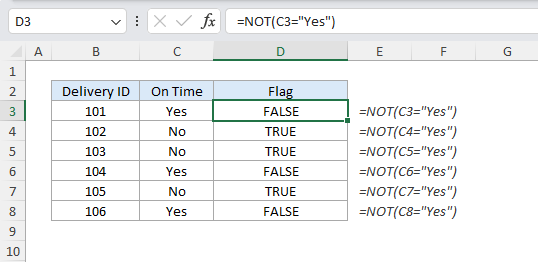
=NOT(C3="Yes")The formula reverses the condition where the result returns FALSE when the delivery is on time.
A company verifies phone numbers and flags entries that are not valid.
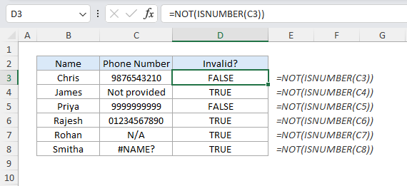
=NOT(ISNUMBER(C3))The ISNUMBER function checks if the phone number entered or present in the dataset is valid, and the NOT function inverts the result. For “Not Provided”, “N/A” and error value, the result is TRUE which indicates as invalid.
A store wants to exclude specific items, for example, discontinued products from the sales report.
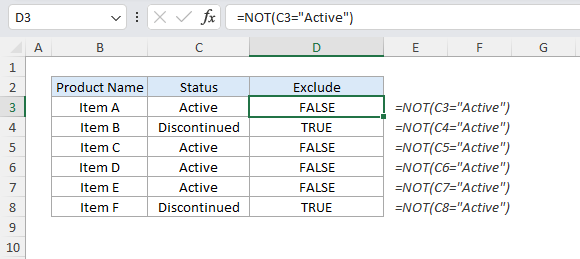
=NOT(C3="Active")The formula checks if all three conditions are met. Rohan meets all the conditions passed, so the result is TRUE. However, Augustin scored 85 in Math but not greater than the first logic and the result is FALSE.
A store wants to give discounts to those customers who either don’t have a membership or haven’t spent more than $500.
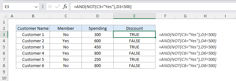
=AND(NOT(C3="Yes"),D3<500)The AND function checks if the customer is not a member and also has not spent above $500. For Customer 1, the customer is a member and also he didn’t spend more than $500 and the result is TRUE.
A factory identifies defective items that either fail inspection or are not properly labeled.
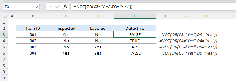
=NOT(OR(C3="Yes",D3="Yes"))The OR function evaluates if spending exceeds $500 or if the item purchased exceeds 10, and the AND function ensures the customer is a member. Aman qualifies and the formula returned Eligible and as Anjali does not, it returned blank.
A project manager wants to prioritize the tasks that are not marked as completed.
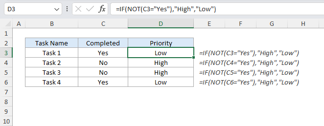
=IF(NOT(C3="Yes"), "High", "Low")The OR function checks if the employee attended on either Saturday or Sunday, and the NOT function reverses the result. Vijay is marked as present, while Meera is marked as absent.
The NOT function simplifies the logical tests by inverting the results and is useful when you want to exclude specific conditions, validate data or combine with other functions for complex scenarios.
No comments yet. Be the first to comment!
Free offline Android app to learn Excel formulas, functions & shortcuts anytime, anywhere!
Download Free AppUse F2 to edit a cell without double-clicking on it.