The VLOOKUP Function in Excel
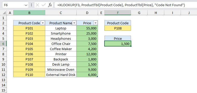
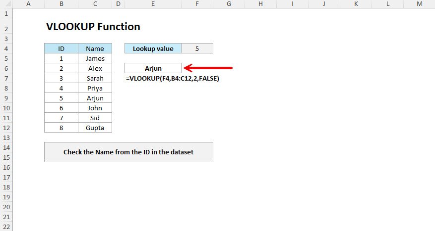
The VLOOKUP function in Excel looks for a value in the first column of a table and gives you back information from another column in the same row.
The XLOOKUP function in Excel is newly introduced in the latest version of Excel, which is a powerful replacement for older lookup functions like VLOOKUP, HLOOKUP, and LOOKUP. It allows you to search for a value in a range or array and return a corresponding value from another range, with much more flexibility and fewer limitations.
=XLOOKUP(lookup_value, lookup_array, return_array, [if_not_found], [match_mode], [search_mode])
Think of XLOOKUP like a smarter version of VLOOKUP that removes old restrictions where it supports only looking for the value in the first column of your dataset and then returning results from the right, as XLOOKUP can return and look from anywhere in the range.
You can use XLOOKUP for:
If you have older versions of Excel, find out complete guide on VLOOKUP
You have employee IDs in column B and want to find the department from column D.
=XLOOKUP(F3, B2:B12, D2:D12, "Not Found")
If you type an employee ID into cell F3, XLOOKUP scans the ID list in column B and fetches the matching department name from column D. If the ID isn’t found, instead of showing #N/A, you’ll see a clear message like “Not Found.”
You need product prices from a product list when you type in product codes.
=XLOOKUP(F3, ProductTbl[Product Code], ProductTbl[Price], "Code Not Found")
When you type a product code in F3, XLOOKUP searches the Code column and returns the Price. If the product code doesn’t exist, it shows "Code Not Found".
A teacher wants to convert numeric scores into grades using a grade table.
=XLOOKUP(C3, GradeTbl[Score], GradeTbl[Grade], , -1)
The student’s score in C3 is compared with the grade table. By using -1 (Exact match or next smaller item), scores that don’t match exactly still fall into the correct grade range.
A sales team earns commissions based on their sales range.
=XLOOKUP(C3, CommissionTbl[Sales Amount], CommissionTbl[Commission Rate], , -1)
If someone sold $18,000 and the exact number isn’t in the table, XLOOKUP finds the next smaller sales bracket and returns the correct commission rate.
You want a polished report without ugly error messages.
=IFERROR(XLOOKUP(C9,B2:B7,C2:C7),"Employee Not Found")
If the employee ID isn’t found, Excel shows "Employee Not Found" instead of an error.
You only know part of a product name but want to look it up.
=XLOOKUP("*"&F3&"*", ProductWildcardTbl[Product Name], ProductWildcardTbl[Price], "No Match", 2)
The 2 (Wildcard match) option allows partial matches, so typing "Phone" will match "Smartphone" or "Headphone".
You want to find the last sale made by a salesperson instead of the first.
=XLOOKUP(B11, SalesTable[Salesperson], SalesTable[SaleDate],"No Record",0,-1)
The -1 search mode tells Excel to search from bottom to top, so you get the last matching record.
Feel free to download and practice to master the XLOOKUP funciton in Excel.
XLOOKUP is one of the most powerful functions in modern Excel and makes your formulas simpler, smarter, and cleaner. Whether you’re working with employee databases, product catalogs, or financial models, XLOOKUP can save you time and reduce formula errors.
No comments yet. Be the first to comment!
Press Ctrl+Shift+L to quickly add filters to your data range.