25 Essential Excel Shortcuts Every Data Analyst Should Know
Ever wished you could analyze data in Excel at the speed of light? With these 25 essential shortcuts, you'll work smarter, not harder. Let me show you...

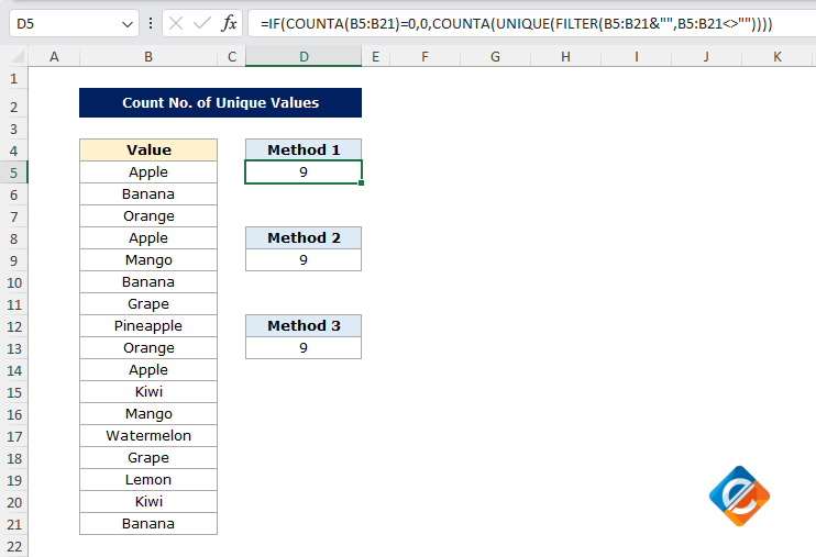
As you know, Excel is a powerful tool, but sometimes it can be confusing, especially when we need to perform a specific task such as counting the unique values. You can use the UNIQUE function to return the unique values, but let’s learn three different formulas to count unique values in Excel which will just return us the unique number.
To count the unique values from your dataset is a crucial and most required task in data analysis. Assume you have a list of customers or products, and you need to find out how many unique entries are there. This could be very useful for inventory tracking, customer profiling, or even useful in financial reporting. Instead of manually checking, we can rely on a few Excel formulas to do the work for us. Below is a step-by-step guide with examples, so even if you are new to Excel, you can understand and use these formulas effectively.
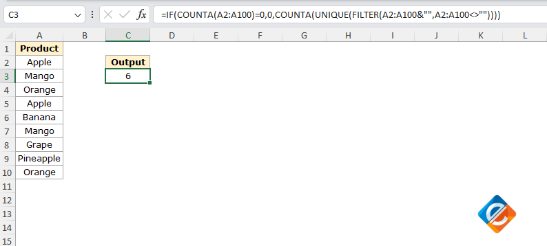
=IF(COUNTA(A2:A100)=0,0,COUNTA(UNIQUE(FILTER(A2:A100&"",A2:A100<>""))))
This formula is very efficient when you have blank cells in your dataset because it will filter the blank cells automatically and return only cells that have data. It is especially useful in newer versions of Excel (Excel 365 and Excel 2019), where the UNIQUE and FILTER functions are available.
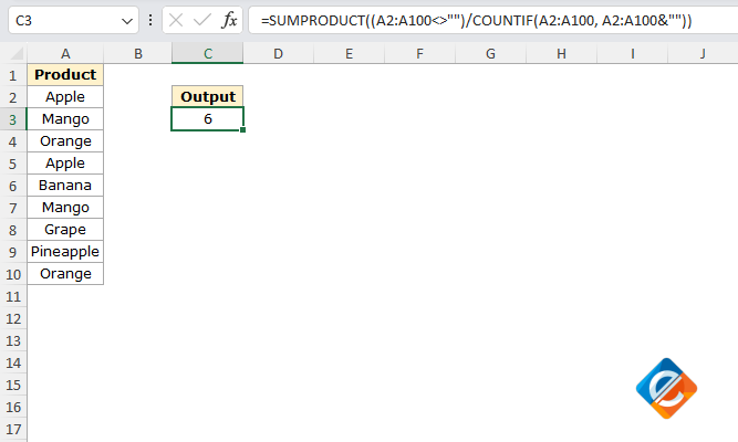
=SUMPRODUCT((A2:A100<>"")/COUNTIF(A2:A100, A2:A100&""))
This formula works in all the versions of Excel, so it is a perfect solution for those using older versions of Excel like Excel 2016 or 2013.
=SUM((A2:A100<>"")/COUNTIF(A2:A100, A2:A100&""))This formula is also compatible with all versions of Excel and is a handy alternative if you want to use SUM instead of SUMPRODUCT.
No comments yet. Be the first to comment!
Free offline Android app to learn Excel formulas, functions & shortcuts anytime, anywhere!
Download Free AppUse Ctrl+T to convert your data range into a formatted table instantly.