Freeze Panes is a most useful feature in Excel which allows you to lock the Rows and Columns in one place so you can scroll through the rest of the data which makes it very easy to read and navigate the column header. You can free more than one row and column.
For example, if you want to keep the column headers of your employee database such as name, address, mobile number, email address etc. fixed at the top while scrolling through hundreds of employees in rows, Freeze Panes can help you achieve it. Similarly, if you want the first column to be locked at the left side of your Excel screen so you can scroll horizontally through the data, Freeze Panes can easily do it.
Why is Freeze Panes Important?
Easily navigate through your data so you do not need to scroll up and down to identify what column you are looking at as Freeze Panes locks your headers.
Once you have locked your column or row headers, it will save you time as you won’t be checking your labels every time.
It also helps you structure your data especially when dealing with large datasets.
Options of Freeze Panes in Excel
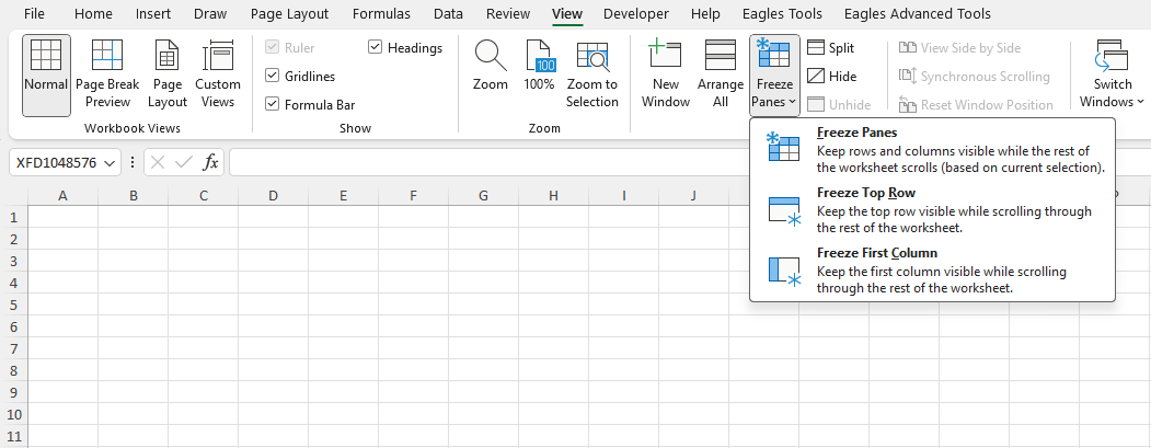
Excel allows you to freeze your rows and columns in three different ways based on your requirements:
Freeze Top Row: This locks the first row of your data which is useful for keeping the headers of your dataset visible by scrolling up or down.
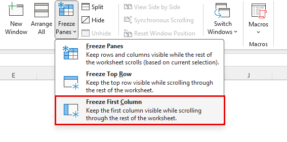
Freeze First Column: This locks the first column of your data which is ideal if you are scrolling right to left.
Freeze Panes: Suppose you want to freeze a combination of both, this will let you freeze multiple rows, multiple columns or also both as per your need.
How to Use Freeze Panes in Excel
1. Freezing the Top Row
It is very important to freeze the column headers while doing data analysis or working with data entry in Excel if you are maintaining a large dataset. Follow the below steps to freeze the top row of your worksheet:
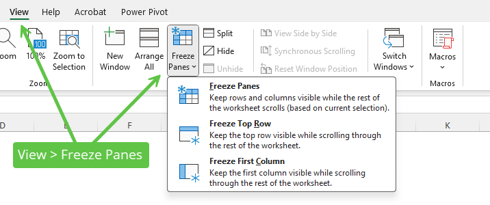
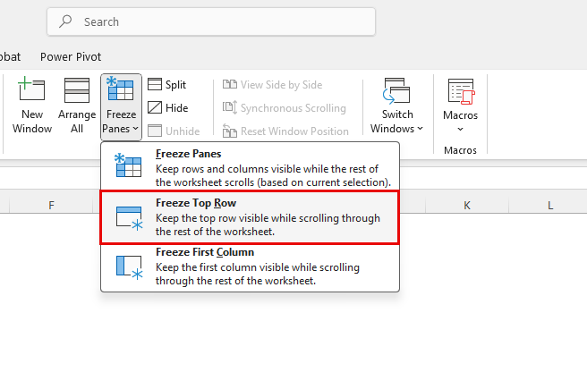
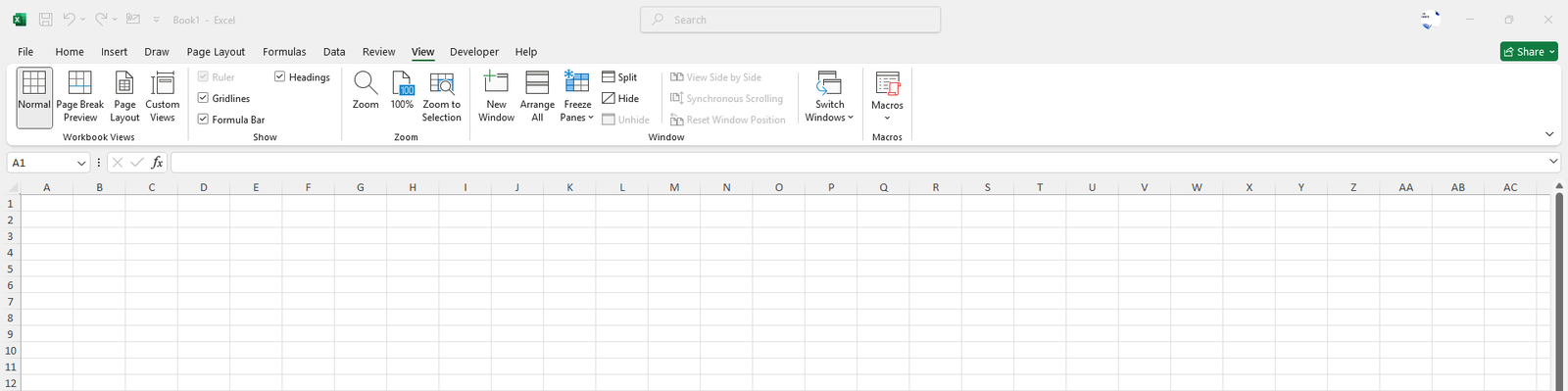
In your worksheet, go to the View tab
Navigate to the Window group, and select Freeze Top Row under the Freeze Panes menu.
The first row is now frozen and when you scroll down, the top row will stick at the same place so it is easy to understand which value belongs to which column.
2. Freezing the First Column
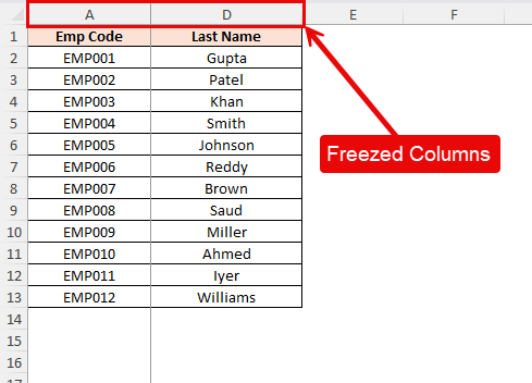
This is a handy option when you are dealing with an employee database or sales database where you want to retain the Employee Code or Employee Name or Invoice No in the first column. Follow the below steps to freeze the first column of your worksheet:
Navigate to the View tab and under the Window group click on Freeze Panes.
Select Freeze First Column.
Now, as you scroll horizontally until the last column of Excel, the first column will stick at the right side of the Excel screen.
3. Freezing Multiple Rows and Columns
If you want to freeze more than one row or column at the same time, you can use this feature to get your desired output.
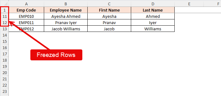
If you want to freeze the first four rows in your dataset, select the 5th row and Under the View Tab, go to Freeze Panes and click on Freeze Panes.
The first four rows are now locked from your dataset.
For example, if you want to freeze both of your rows and columns, follow as below:
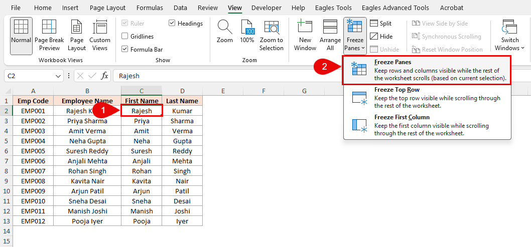
Select the cell that is under your last desired row and last desired column to freeze. For example, if you want to freeze the first two rows and the first column, then select cell C2.
Click on Freeze Panes under the View Tab as shown in below image.
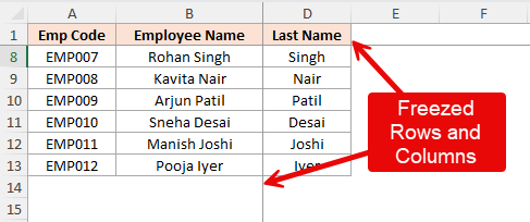
This will freeze column A and column B and also row 1 so you can scroll freely through the rest of your data. It will be helpful when you want to keep your headers fixed in one place and also your Invoice Number or in shown examples Employee Code and Employee Name to scroll towards the right.
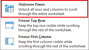
How to Unfreeze Panes
To quickly unfreeze the rows or columns follow the below steps:
Go to the View tab.
Under the Window group, go to Freeze Panes.
Select Unfreeze Panes.
Real-Life Uses of Freeze Panes
Let’s look at some of the practical scenarios where Freeze Panes can be very helpful:
Financial Reports: When working with financial reports that include various tabs and datasets such as monthly revenue, incomes and expenses, profit and loss, freezing the top row which has headers or the name of months or freezing the first column which has categories, types or department names makes it easier to compare data without losing track of what each amount represents.
Attendance Sheets: As we saw in our examples, if you have a list of Employee Codes or Employee Names, freezing the first column or first two columns helps you scroll to see attendance for every month so you don’t lose track of which employee you are looking at.
Project Tracking: Freezing the first row which contains task details ensures the name of the task is visible when you are scrolling through the deadlines or date of completion.
Tips for Using Freeze Panes
Below are a few tips you can use:
When freezing multiple rows or columns in your worksheet, make sure you are selecting the correct cell. Everything towards the left and above will be locked or frozen.
If you are working on large datasets, Freezing the rows and columns helps you keep important information visible when scrolling.
Don’t forget to unfreeze the panes if you no longer require them to avoid further confusion when navigating through the sheet.
Conclusion
A most required feature in Excel simplifies the workflow by keeping the required rows and columns visible when working on large spreadsheets such as managing financial data, attendance tracking etc.
The View Tab offers you a variety of options that help you control the way you want your workspace to be displayed within the workbook based on your r...
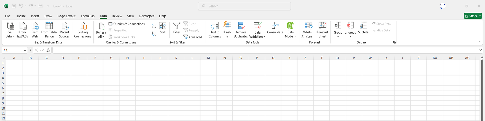
The Data Tab helps you manage, analyze and organize your data efficiently. It is a pack of functionalities such as sorting, filtering, importing and s...
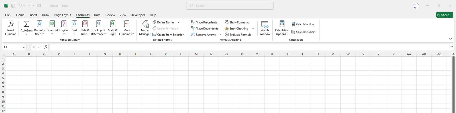
The Formula Tab helps you create, manage and analyze calculations within your workbook. It provides access to a variety of pre-defined functions and t...
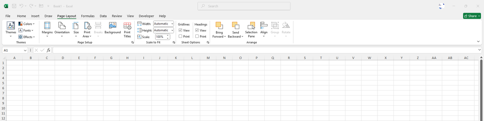
The Page Layout Tab helps you control the appearance and set up the print area to be printed in your worksheets ensuring your data looks clear and pro...